One of the great features that MS Excel has is the capability to restrict (validate) the input into certain cells. The name of this feature in MS Excel is Data Validation.

A few examples of this is to restrict the values of cells to be

• text of a certain length
• numbers within range
• a selection from a list of possible values,
• and many more…

The data validation feature is found in the ‘Data’ tab as shown below.

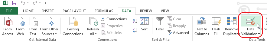
Figure 1: Data Validation Menu Option

In order to illustrate the different types of data validation options. We’ll use the following data entry form:

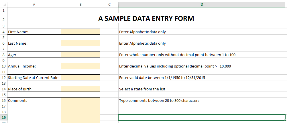
Figure 2: Sample Form

The data validation types shown in this post are:

• Accepting Integer Values Only
• Accepting Decimal Values Only
• Accepting Valid Dates Only
• Accepting Values From Lists
• Accepting Text Of A Certain Length Only
• Validating Entries With Formulas: Accepting Text Only Values
• Validating Entries With Formulas: How To Avoid Duplicate Entries In A Column
• How To Circle Invalid Data

ACCEPTING INTEGER VALUES ONLY

Sometimes it is required that users must type integer values only, as in cell B8 in our sample form. In order to enforce this constraint, we can follow these steps:

1. Click in cell B8.
2. Click on ‘Data’ ‘Data Validation’ ‘Data Validation …’
3. Select ‘Whole number’ from ‘Allow:’ option.
4. Select the criteria from the ‘Data’ option, e.g. ‘between’ and give minimum and maximum values. Your screen should look like the one shown in the figure below.

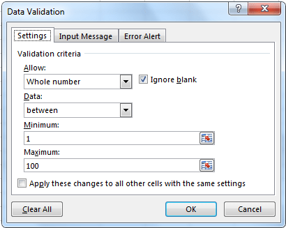
Figure 3: Data Validation Rule (Whole Number)

1. Click ‘OK’.

Now users will be not allowed to type anything but whole numbers in B8. If you enter something different from whole numbers or a whole number outside the specified range, then you’ll get an error message like this one.

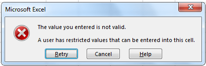
Figure 4: Default Error Dialog Box

We can customize this window to display a more meaningful message following these steps:

1. Click in cell B8.
2. Click on ‘Data tab’ ‘Data Validation’ ‘Data Validation …’
3. You will see the validation rule previously defined
4. Click on the ‘Error Alert’ tab.
5. Select ‘Stop’ from ‘Style:’ combo box.
6. Type a meaningful text like ‘Invalid Data Entered’ in ‘Title’ textbox.
7. Type the message to be displayed when an invalid data is entered in text area provided under ‘Error Message’.
8. Your window should look like as shown in the figure below.

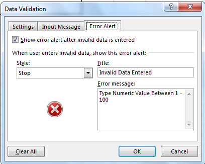
Figure 5: Customized Error Alert

1. Click on ‘OK’.

Now if you enter an invalid data in cell B8, then you will receive an error message as shown in figure 6 below.

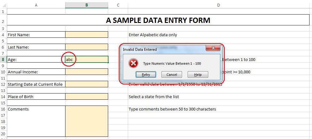
Figure 6: Error Alert (Whole Number)

ACCEPTING DECIMAL VALUES ONLY

Sometimes it is required that user must type decimal values only as required in cell B10 in our sample form. In order to enforce this constraint, we can follow these steps.

1. Click in cell B10.
2. Click on ‘Data tab’ ‘Data Validation’ ‘Data Validation …’
3. Select ‘Decimal’ from ‘Allow:’ option.
4. Select criteria from ‘Data’ option, e.g. ‘greater than or equal to’ and enter ‘10000’ as ‘Minimum’ value as shown in the figure 7 below.
5. Click ‘OK’.

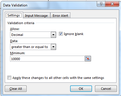
Figure 7: Data Validation Rule (Decimal Number)

Now, if the user enters something different than a decimal number within the acceptance criteria in B10 then an error dialog box is displayed as shown in figure 8 below. This error message is created by following the same steps shown above in figure 5.

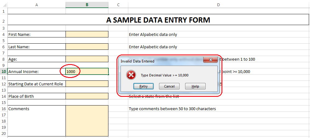
Figure 8: Error Alert (Decimal Number)

ACCEPTING VALID DATES ONLY

You can use data validation for validating dates as well, as required in cell B12 in our sample form. In order to enforce this constraint, we can follow these steps.

1. Click in cell B12.
2. Click on ‘Data tab’ ‘Data Validation’ ‘Data Validation …’
3. Select ‘Date’ from ‘Allow:’ option.
4. Select criteria from ‘Data’ option, e.g. ‘between’ in our case. Enter ‘Start Date’ and ‘End Date’. The values given in ‘Start date’ and ‘End date’ must be valid dates. We can also use formula if required. For example, we can limit the maximum date to the current date as shown in the figure 9 below.
5. Click ‘OK’.

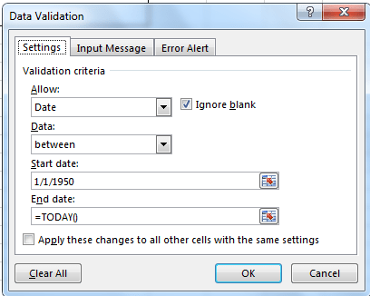
Figure 9: Data Validation Rule (Date)

If a valid date within the acceptance criteria is not entered in B12 then an error dialog box is displayed as shown in figure 10 below. This error message is composed by following the steps mentioned earlier and shown in figure 5.

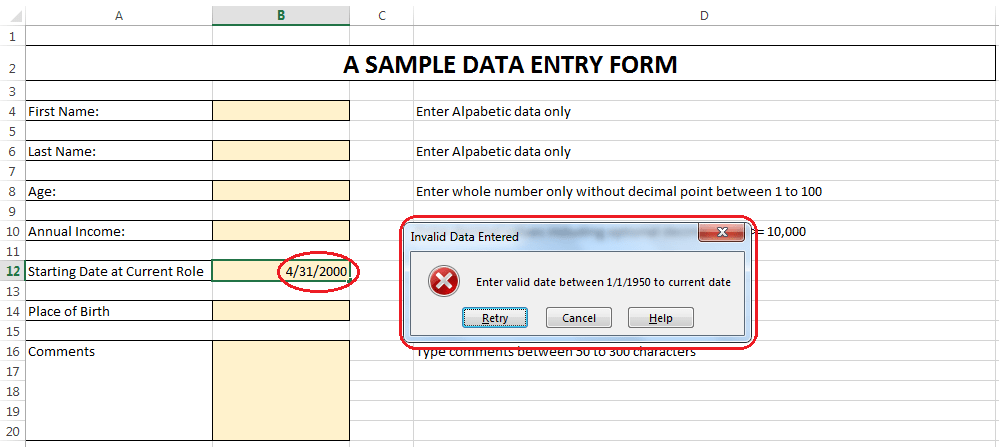
Figure 10: Error Alert (Date)

ACCEPTING VALUES FROM LISTS

In some cases, you want to force the user to enter values from a specific list. In our sample form, user is required to select his place of birth in cell B14 from a predetermined list of places. In order to enforce this constraint, we can follow the steps given below.

1. Click in cell B14.
2. Click on ‘Data tab’ ‘Data Validation’ ‘Data Validation …’
3. Select ‘List’ from ‘Allow:’ option.
4. Select the source from where the data will be displayed in the form of a drop-down list. The source can be a cell range from the same sheet or from a different sheet of the same workbook. For example in our case, there is a sheet called ‘States’ with names of all states of US located in the range A1:A50, therefore the cell reference to be used in our form is =States!$A$1:$A$50 as shown in the figure 11 below.
5. Click ‘OK’.

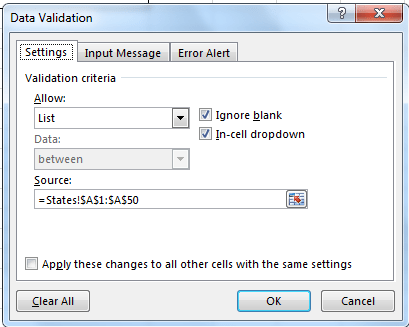
Figure 11: Data Validation Rule (List)

Now user will not be allowed to type anything in B14 but the values on the list selected. Users can either manually type the entries or select them from the dropdown-list that appears when the cell is selected. If a value that is not in the list is typed then an error dialog box is displayed as shown in figure 12 below. This error message is composed by following the steps mentioned earlier and shown in figure 5.

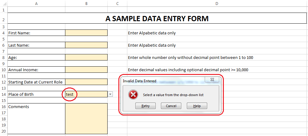
Figure 12: Error Alert (List)

There are several cool things that can be done with lists in Excel, for example, creating expandable lists, or dependent lists.

Click here to know more about lists!

ACCEPTING TEXT OF A CERTAIN LENGTH ONLY

If you want to restrict the length of a text entry you can do it as well. For example, in our sample form, user is required to type comments between 20 to 300 characters. In order to enforce this constraint, we can follow the steps given below.

1. Click in cell B16.
2. Click on ‘Data tab’ ‘Data Validation’ ‘Data Validation …’
3. Select ‘Text length’ from ‘Allow:’ option.
4. Select criteria from ‘Data’ option, e.g. ‘between’ in our case. Enter ‘Minimum’ and ‘Maximum’ values as shown in the figure 13 below.
5. Click ‘OK’.

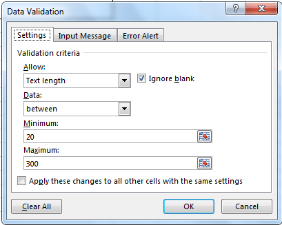
Figure 13: Data Validation Rule (Text Length)

User will be required to type text between 20 to 300 characters in B16. If user types less than 20 or more than 300 characters in B16 then an error dialog box will be displayed as shown in figure 14 below. This error message is composed by following the steps mentioned earlier and shown in figure 5.

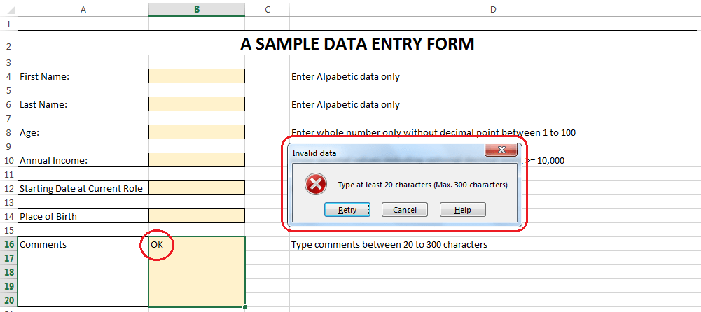
Figure 14: Error Alert (Text Length)

VALIDATING ENTRIES WITH FORMULAS : ACCEPTING TEXT ONLY VALUES

On top of all the possible options shown for data validation, you can also use a formula that return a logical value to validate entries. For example, let’s say you want make sure that only text is entered in a cell. You can use the function ISTEXT which will return TRUE if the entry is text and FALSE otherwise. In order to enforce this constraint, we can follow these steps.

1. Click in cell B4.
2. Click on ‘Data tab’ ‘Data Validation’ ‘Data Validation …’. You will see a window as shown in figure 15 below.
3. Select ‘Custom’ from ‘Allow:’ option and type ‘=ISTEXT(B4)’ in ‘Formula:’. Keep ‘Ignore Blank’ checked if you want to ignore blank values in cell B4.

Notice that the cell entered in the formula is the cell where you’re creating the data validation rule.

4. Click ‘OK’.

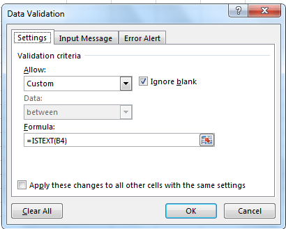
Figure 15: Data Validation Rule (Text Only)

Now the user will be only allowed to type text data in B4. If numbers are entered without alphabetic characters then data will not be accepted and an error dialog box is displayed as shown in figure 16 below. This error message is composed by following the steps mentioned earlier and shown in figure 5.

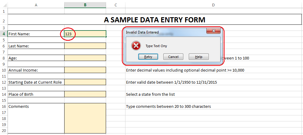
Figure 16: Error Alert (Text Only)

Repeat the same steps for cell B6 to accept valid data against ‘Last Name’.

VALIDATING ENTRIES WITH FORMULAS : HOW TO AVOID DUPLICATE ENTRIES IN A COLUMN

Another possible application of validating entries with formulas is to avoid duplicate entries in a column. For example, let’s say we have a column in our sheet where unique US state names need to be entered. This constraint can be enforced by following the steps given below.

1. Select the cell range where the duplicate entries will not be allowed, e.g. A1:A200 as an example.
2. Click on ‘Data tab’ ‘Data Validation’ ‘Data Validation …’
3. Select ‘Custom’ from ‘Allow:’ option.
4. Type the formula ‘=COUNTIF($A$1:$A$200,A1)=1’ in ‘Formula’ option. Your window should look as shown in figure 20 below.
5. Click ‘OK’.

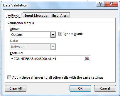
Figure 17: Data Validation Rule (Restrict Duplicate Values)

Now user will not be allowed to enter duplicate values in the range specified (A1:A200 in our example). If user enters a duplicate value then an error dialog box is displayed as shown in figure 18 below. This error message is composed by following the steps mentioned earlier and shown in figure 5.

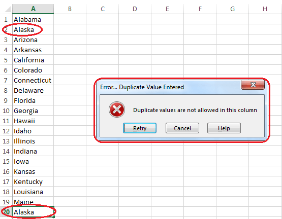
Figure 18: Error Alert (Duplicate Value)

HOW TO CIRCLE INVALID DATA

What happens when you apply a data validation rule to cells that already contain values?

Suppose we have some values in a sheet as shown below.

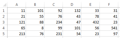
Figure 19: Sample Data to Circle Invalid Data

and you want to restrict the entries in that range to be between 1 and 100. The first step would be to create the validation rules following the steps shown below:

1. Select the range (A1:F5 in our case).
2. Click on ‘Data tab’ ‘Data Validation’ ‘Data Validation …’
3. Select ‘Whole Number’ from ‘Allow:’ option.
4. Select criteria from ‘Data’ option, e.g. ‘between’ in our case. Enter ‘Minimum’ and ‘Maximum’ values as shown in the figure 20 below.
5. Click ‘OK’.

Figure 20: Data Validation Rule to Circle Invalid Data

Once you apply the validation rule, Excel won’t delete the values that don’t comply with rule, instead it can help you identify where are those values.

In order to do this, follow these steps:

1. Click again on ‘Data tab’ ‘Data Validation’ ‘Circle Invalid Data’.
2. You will see that all the invalid values (outside 1 and 100) are circled as shown in the figure 21 below.

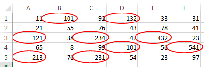
Figure 21: Invalid Data Encircled

You can clear the circles by clicking ‘Data tab’ ‘Data Validation’ ‘Clear Validation Circles’.