Yes, you read the title of this post correctly, you can calculate the median and lots of other functions in Excel PivotTables besides the regular options.
If you’re a regular user of Excel PivotTables you might know you can change the summary function:
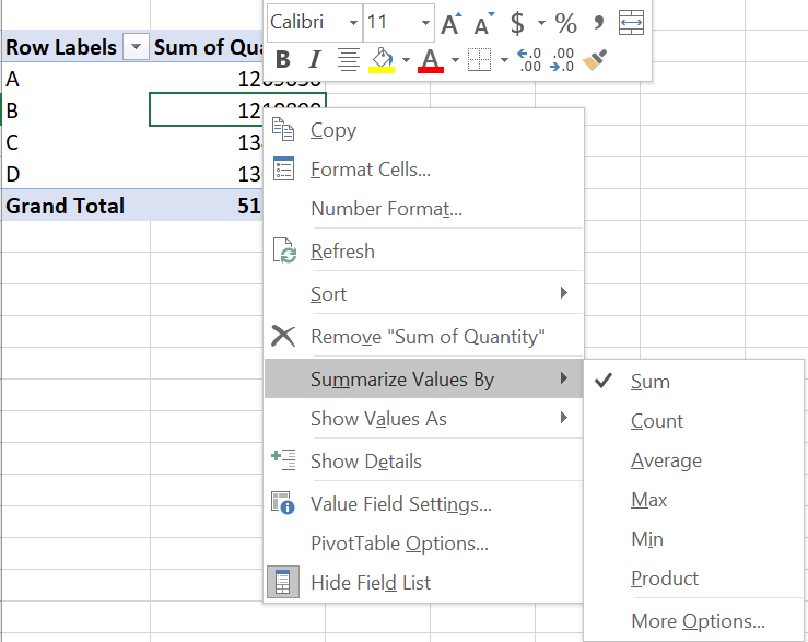
Just right-click inside of the PivotTable → Go to Summarize Values By → Select the summary function
Change summary function in PivotTable
If you click on More Options…, you can select other functions such as Standard Deviation and CountNumbers. But, what if you need something different such as the median? That’s when Power Pivot comes into play.
Power Pivot is an Excel built-in feature (for Excel 2013 and later) that allows you to significantly extend the capabilities of regular PivotTables. For example, with Power Pivot you can use information from multiple tables without having to join it into a single table. Also, you can use lots of summary functions that are not available in regular PivotTables (e.g. Median). Note: The median function is only available in Power Pivot for Excel 2016.
Check this 5 min video below to get more information about Power Pivot
To show how to calculate the median (or another measure) in PivotTables, I’ll use a sample dataset that contains shipping data. The dataset contains the following columns:
Order Number: ID of the order
Distribution Center: Location from where the order is shipped
Quantity: Number of items shipped in the order
Order Date: Date when the order was placed by the customer
Delivery Date: Date when the order was delivered to the customer
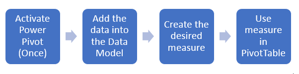
The process to calculate the median (or any other function) in PivotTables is as follows:
Create a measure in Power Pivot
» Activate Power Pivot
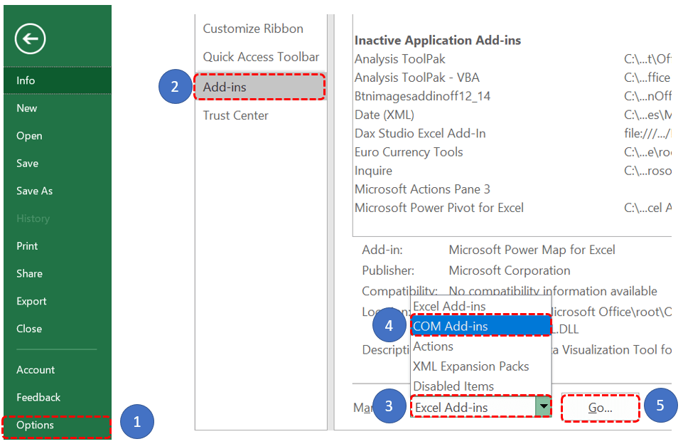
The activation of Power Pivot must be done once. These are the steps to do it:
Go to File → Options → Add-ins
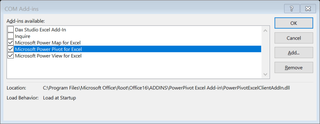
Then select COM Add ins from the drop down and click on GoEnable PowerPivot in Excel
Check the checkbox for Microsoft Power Pivot for Excel and click OKCheck box to activate Power Pivot in Excel
» Load the data into Power Pivot
Place the cursor on any cell within the range that contains the data
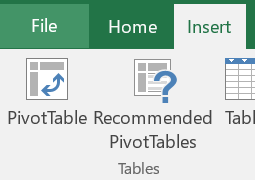
Go to Insert → PivotTableInsert Pivot Table
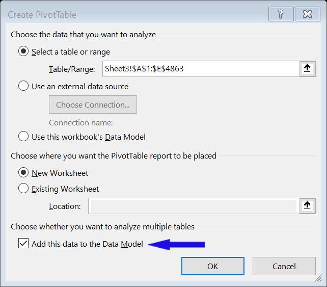
Make sure the range selected is appropriate and check on Add this data to the Data Model.
Click OK.Add data to Excel Data ModelNote: If you’re importing the data from an Excel Table, the Data Model will use the table’s name, otherwise, it will use the name Range for the table. Keep this in mind as it is import for the second example of this post.
» Create the desired measure
Go to the Power Pivot tab → Click on Measures → New Measure
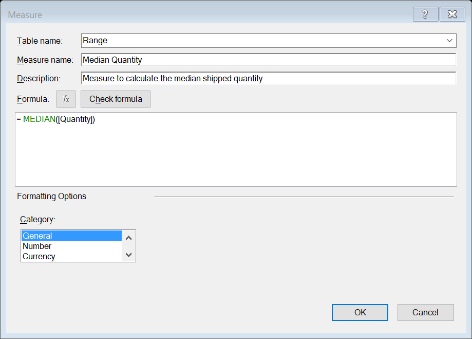
Specify the name of the measure (e.g. Median Quantity)
Enter the formula for the measure. For example, to calculate the median of a column called QUANTITY, enter the formula =MEDIAN([QUANTITY]). Notice the use of brackets to refer to columns.Create a measure with the median
In addition, you can specify the name of the table where the measure will be stored and a description for the measure.
» Use the measure in a PivotTable
You can drag the desired fields and the measure to the PivotTable.
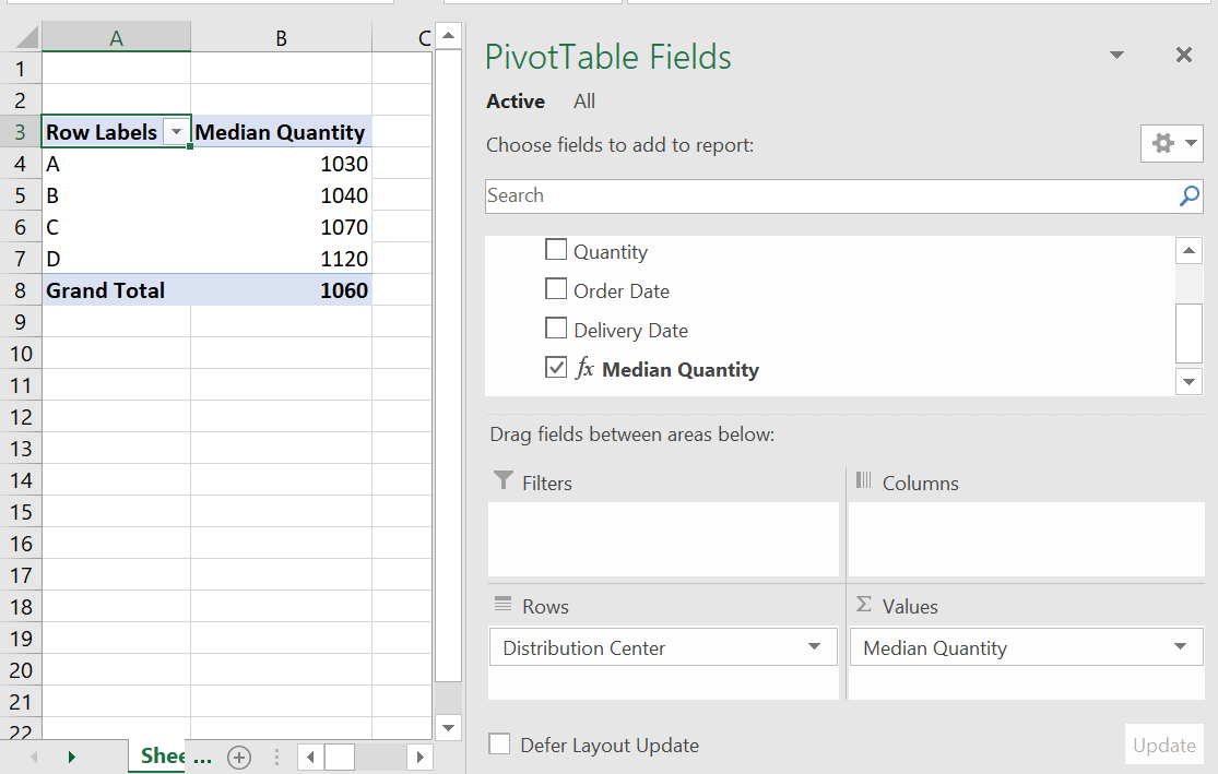
For example, the image below shows a PivotTable with the column Distribution Center in the rows area and the measure Median Quantity in the values area.
Add median to Pivot Table
Calculate the median from row-wise operations
Let’s say you want to calculate the median of the number of days passed from the Order Date to the Delivery Date. This date difference is called leadtime.
There are two ways of doing this:
Create a Leadtime column in the table and then calculate the median of the Leadtime column
Use the function MEDIANX to calculate the leadtime and the median in a single formula
I’ll explain how to use MEDIANX:
All Power Pivot functions ending in X are iterators. Iterator functions can perform an operation for each row of a table.
In general, the syntax for an iterator is:
=FUNCTIONNAMEX(Table, Operation)
In this case, we want to subtract the Order Date from the Delivery Date for each row of the table called Range and then we want to calculate the median of those results.
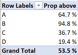
Let’s say there’s a target of having a leadtime (delivery date – order date) of 15 days or less. How would you calculate the percent of orders that had a leadtime greater than 15 days for each of the distribution centers?
The PivotTable should look like this:
Pivot Table with proportion of late orders
If we pick distribution center B, 94.8% of the orders had a leadtime greater than 15 days.
HINT: Read about these Power Pivot functions: COUNTX, AVERAGEX, IF, COUNTROWS, FILTER, BLANK. You don’t need to use all of them to answer the question.
Write your solution in the comments section. By October 15, I’ll share a workbook with all the solutions posted and the names of the people who posted.
Please share this post so more people
can benefit!
Newsletter
Stay up to date with our latest news, receive exclusive deals, and more.