This is the 4th post of a series that covers everything about importing all files in a folder into Excel using a tool called Power Query. Click here to see the series.
The previous scenario covered how to import all Excel files in a folder getting the data below the 9th row. Therefore, the data on all files started at the same row, but what if this is not the case?
What if the files could start at different rows?
For this scenario, we will work with 6 files and each of them start at a different row. See two examples below:
Data of interest in file Sales History – 24796.xlsx starts at row 13
![]()
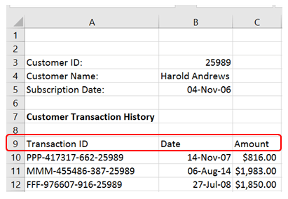
However, in file Sales History – 25989.xlsx data starts at row 9
Download the files from this link to follow along.
To solve this issue, what we will do is to identify the row with the headers on each file and keep all the rows below that one. The process is EXACTLY the same as in the previous example, but rather than deleting a fixed number of rows you will identify the row with headers using a conditional column.
Step 1: Import a single file from the folder
Go to Data → New Query → From File → From Workbook
![]()
Browse for the file and click on Import
Then select the sheet or table to import and click OK
![]()
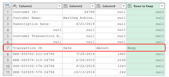
Then go to Add Column → Conditional Column, enter a condition to identify the header row, and click OK. In this case, the header row is located where Column2 is equal to Date.
![]()
The new column, called Rows to Keep, should contain the word “Keep” in the header row
Fill down the column Rows to Keep. Right-click the header of the column → Fill → Down. The table should look like this:

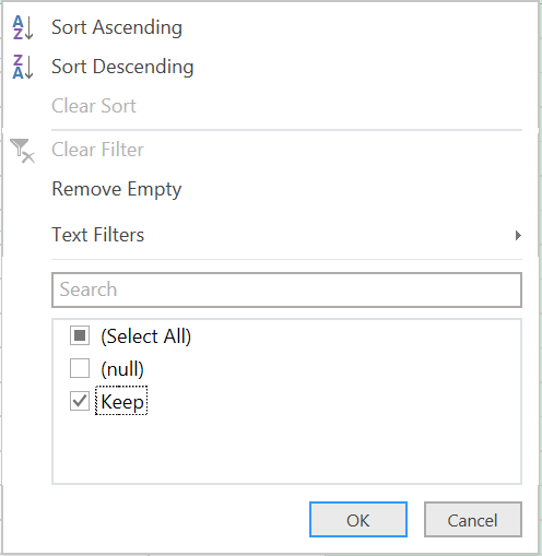
Go to the filter and select the word Keep
Then promote the headers, go to Home → Use First Row as Header
Delete the Keep column
Finally, change the format of the Date column to date (Right-click the header of the Date Column, go to Change Type → Date
Step 3: Create a function
To create a function, go to View → Advanced Editor
![]()
In the Advanced Editor, you will notice that the first line contains the function File.Contents and a fixed path and filename.
![]()
To create the function, we must replace the section in the rectangle above with the parameter name, see below.
The name of the parameter goes at the top surrounded by parenthesis and followed by =>
![]()
Once you create the function click on Done.
Then go to the query name box and rename the function with a new name, e.g., fxGetData.
![]()
Finally, go to File → Close & Load
You should be able to see the function in the Workbook Queries pane along with other queries you have in the workbook.
![]()
Step 4: Apply the function to all files in the folder
Go to Data → New Query → From File → From Folder
![]()
Click on ‘Browse’ and browse for the folder that contain the files, then click OK.
![]()
Once you click OK, press Edit on the next window.
We’re only interested in the Content column, therefore, right-click on the header of the Content column and select Remove Other Columns.
![]()
The go to Add Custom Column → Invoke Custom Function
![]()
Select the function (fxGetData), enter a name for the new column (FileContent), select the columns to pass to the function (Content), and click OK.
If you click on the tables, you’ll be able to see the contents of each one.
Step 5: Expand the contents and load to Excel
Then click on the Expand button in the FileContent column and click OK in the Expand dialog box.
![]()
In the next dialog box, make sure to un check “Use original column name as prefix”.
![]()
Right-click on the header of the column and select Remove
![]()
Change the type of the Date column to date and load the data to the workbook.
That’s All!!!
Click here if you want to see the other posts in the series.
Want to continue learning about automating your data preparation processes?? Subscribe to the blog.