In this post, I’ll show how to create a simple model to predict if a customer will buy a product after receiving a marketing campaign.
Before I get into the example, I’ll briefly explain the basics about the model I’ll use (Logistic Regression).
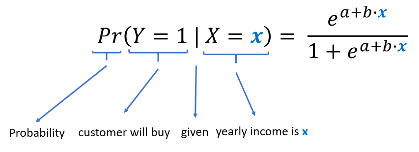
As shown in the image below, you want a model (function) that will get the characteristics of a customer and/or marketing campaign and predict if the customer will buy.
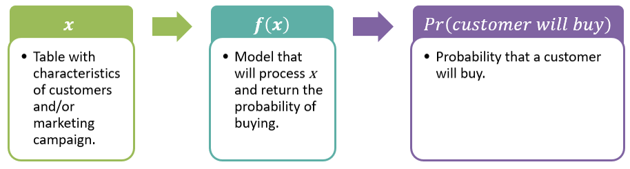
Once you get the probability, you can define a cutoff value to predict if the customer will buy. For example, you can say that if the probability of buying is greater than 0.5 then the prediction will be that the customer will buy.
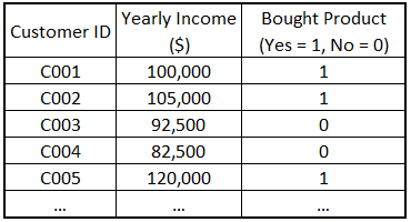
To make these concepts easier to explain let’s consider a toy problem where you only have one customer characteristic (yearly income) and you want to predict if the customer will buy.
A subset of the data I’ll use is presented below:
Download the data from this link.
Here’s a simple plot of the data
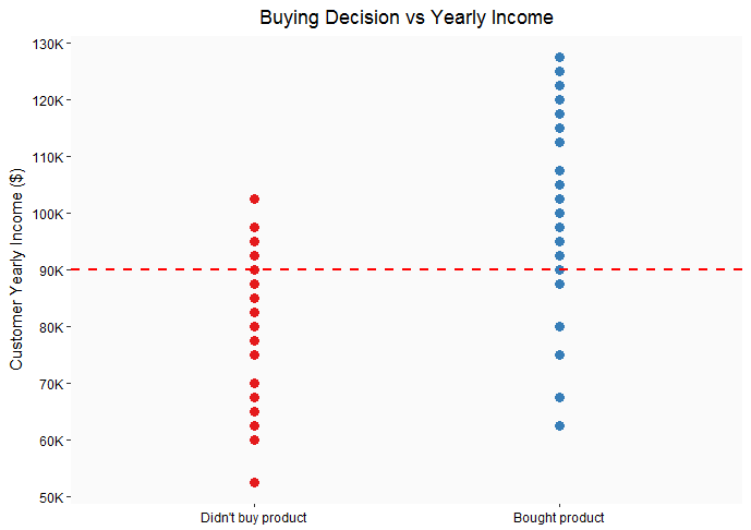
As you can see from the plot, customers who bought the product tend to have higher income (> $90K/year). Similarly, customers who didn’t buy the product tend to have lower income (< $90K/year).
Modeling
We want a model to predict the probability of buying a product based on the yearly income of the customer.
One way of creating this model is to use logistic regression. The following figure shows the true buying decisions for each customer (filled points) and the predicted probabilities of buying given by the logistic regression model (empty points). In this case, the cutoff is 0.5, therefore probabilities greater than 0.5 are classified as WILL BUY (blue) and below 0.5 are classified as WILL NOT BUY (red).
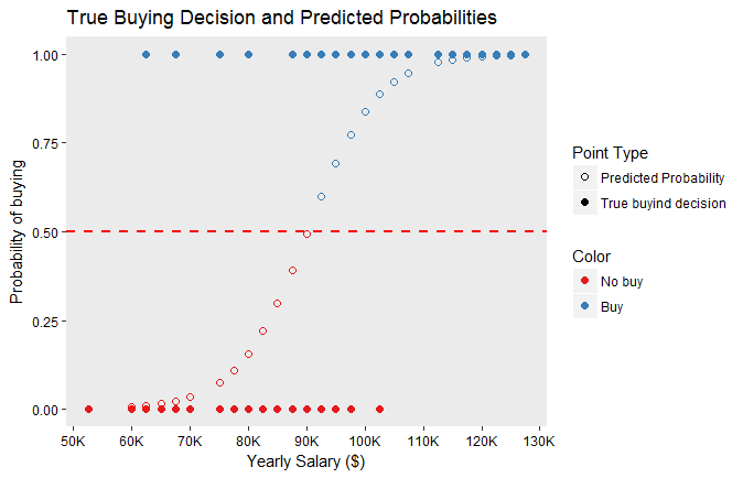
As shown in the previous figure, the model seems to be working well. For customers most customers who bought the product, the predicted probability of buying is above the cutoff value (0.5), therefore, the prediction is that they will buy.
If you’re more mathematically inclined, the equation used to calculate the predicted probabilities shown on the previous figure is as follows:
Once you have obtained the values of the coefficients (a and b) [R can do this for you], you can predict the probability of buying for a customer by substituting its corresponding yearly income.
For example, if the values of the parameters are a = -14.98 and b = 0.000166, and the yearly income for a customer is 105,000; then the predicted probability is calculated as follows:
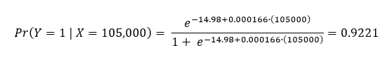
Assuming a cutoff value of 0.5, since the probability (0.9221) is greater than the cutoff value (0.5), the prediction would be that the customer will buy the product.
Don’t worry, you won’t have to do this manually. This link contains the R code to get the data, create the graphs and models, and make the predictions.
Note: To learn more about the application of logistic regression to marketing, read Section 9.2 of the book R for Marketing Research and Analytics (Chapman, 2015).
Real Example: Logistic Regression applied to telemarketing
Now that you know the basics, let’s move to a more realistic example. This example comes from the paper: A Data-Driven Approach to Predict the Success of Bank Telemarketing (Moro et Al., 2014) [Link]. The data set for the example contains information about customers and marketing campaigns for several telemarketing campaigns for a Portuguese banking institution.
The goal here is to predict if a customer will subscribe to a term deposit (buy a product) after receiving a telemarketing campaign.
Data Description
The variables included in the data are grouped as follows:

Download the data from this link, you’ll need it to follow the next steps.
Modeling Steps
I’ll use the caret package to create the model. This is a package with lots of functions to streamline the predictive modeling processes.
Step 1: Import and clean the data
Usually the data cleaning part takes a lot of time and involves several steps such as fixing formatting issues, correcting missing or erroneous values, and standardizing categorical columns.
I won’t cover data cleaning in this post, however please bear in mind the importance of cleaning and plotting the data before going into modeling.
The code below shows how to import the data and to explore each variable using the summary function:
[code lang="r"]
### Import Data ###
setwd(choose.dir(caption = "Select the folder with the telemarketing data"))
data = read.csv("bank telemarketing data.csv")

#Number of rows
nrow(data)

#Explore variables
summary(data)

[/code]
Step 2: Split the data in a training and test set
The goal of creating a predictive model is to make predictions about new data. If you use all data available for creating the model, you won’t be able to test the performance of the model with a data set that was not used to create it. Therefore, is good to split the original data set in training and test sets. The training set will be used to create the model and the test set to evaluate the performance of the model in an unseen data set.
In this example, I’ll use 70% of the data for the training set and 30% for the test set.
Here’s the code:
[code lang="r"]
library(caret)
### Create training and test sets ###
inTrain = createDataPartition(y = data$y, #Variable that we want to predict
                              p = 0.7, #Proportion of values in training set
                              list = FALSE) #Return a vector of indices

#Create training and test sets
TrainingSet = data[inTrain, ]
TestSet     = data[-inTrain, ]
[/code]
The createDataPartition function returns the set of indices for the rows of the data set that will be included in the training set.
Step 3: Model creation
I’ll use the train function from the caret package to fit the logistic regression model. This function is very versatile and capable of fitting many different models. You just need to specify the model type using the method parameter and the additional details required by the method selected.
Examples:
![]()
The train function also has parameters for doing model tuning. For more details about this or other functions from the caret package, check the package vignette.
Here’s the code to fit the logistic regression model:
[code lang="r"]
### Train model ###
mod = train(y ~ .,
            data = TrainingSet,
            method = "glm",
            family = "binomial")
[/code]
Logistic regression is a generalized linear model (glm) with a binomial family. To read more about fitting and analyzing GLMs, check the book: An Introduction to Generalized Linear Models (Dobson, 2008)
Step 4: Check model performance
Now that we have the model, let’s check its performance on the training and tests sets. The most basic performance measure is Overall Accuracy which is the proportion of times the models predicts correctly.
See the code below:
[code lang="r"]
### Get predictions ###
ptest  = predict(mod, newdata = TestSet)
ptrain = predict(mod, newdata = TrainingSet)

### Accuracy ###

#Accuracy for training set
mean(ptrain == TrainingSet$y)

#Accuracy for Test set
mean(ptest == TestSet$y)
[/code]
The accuracy for both the training and test sets are: 91.16% and 91.24%. You might get slightly different values.
Pretty good accuracy, right?
PLEASE DON’T FALL INTO THIS TRAP!!!
These high accuracy values might be due to class imbalance in the data sets.
The class imbalance problem
Class imbalance happens when the relative frequency of one class (e.g. customers who bought the product) is very low when compared to the other (e.g. customers who didn’t buy the product). This happens in many scenarios:
- Digital marketing: Click through rate (Only a small proportion of people click on the links)
- Banking: Fraud detection (Most transactions are non-fraudulent)
- Healthcare: Cancer prediction (Almost all tissues analyzed don’t have cancer cells)
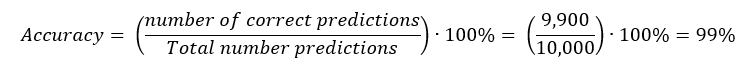
The calculation of prediction accuracy can be problematic in imbalanced data sets. Let’s see an example for an email campaign:
Imagine you have a crappy model that always predicts that customers WILL NOT click on the links sent to them. In other words, this model will FAIL ALL predictions for customers who clicked on the links.
Suppose we are evaluating the accuracy of this model with an imbalanced data set (Out of 10,000 customers only 100 clicked):
 For this same model, let’s evaluate the accuracy for a balanced data set (Out of 10,000 customers; 5,000 cliked):
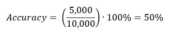
As you can see, the high accuracy observed with the imbalanced data set is due to the nature of the data set and not the performance of the model. Fortunately, you can use other metrics to measure the performance of models such as Precision, Recall, and Area Under the ROC curve.
Unfortunately, class imbalance has negative effects in the true performance of the models. In other words, if you train the models using an imbalanced data set this might cause the models to predict incorrectly in a frequency higher than expected.
What can you do if you have to deal with the common problem of class imbalance? Easy, subscribe to the blog! I’ll write another post about multiple ways of dealing with class imbalance.